clc
clear all
clc
clf
disp('This program compares results from the')
disp('exact solution to 2nd order Runge-Kutta methods')
disp('of Heuns method, Ralstons method, Improved Polygon')
disp(' method, and directly using the three terms of Taylor series')
fcnstr='sin(5*x)-0.4*y' ;
x0=0;
y0=5;
xf=5.5;
n=10;
f=inline(fcnstr) ;
syms x
eqn=['Dy=' fcnstr]
exact_solution=dsolve(eqn,'y(0)=5','x')
xx=x0:(xf-x0)/100:xf;
yy=subs(exact_solution,x,xx);
yexact=subs(exact_solution,x,xf);
plot(xx,yy,'.')
hold on
h=(xf-x0)/n;
a1=0.5;
a2=0.5;
p1=1;
q11=1;
xr=zeros(1,n+1);
yr=zeros(1,n+1);
xr(1)=x0;
yr(1)=y0;
for i=1:1:n
k1=f(xr(i),yr(i));
k2=f(xr(i)+p1*h,yr(i)+q11*k1*h);
yr(i+1)=yr(i)+(a1*k1+a2*k2)*h;
xr(i+1)=xr(i)+h;
end
y_heun=yr(n+1);
et_heun=abs((y_heun-yexact)/yexact)*100;
hold on
xlabel('x')
ylabel('y')
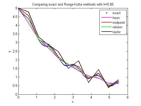
title_name=['Comparing exact and Runge-Kutta methods with h=' num2str(h)] ;
title(title_name)
plot(xr,yr, 'color','magenta','LineWidth',2)
a1=0;
a2=1;
p1=1/2;
q11=1/2;
xr(1)=x0;
yr(1)=y0;
for i=1:1:n
k1=f(xr(i),yr(i));
k2=f(xr(i)+p1*h,yr(i)+q11*k1*h);
yr(i+1)=yr(i)+(a1*k1+a2*k2)*h;
xr(i+1)=xr(i)+h;
end
y_improved=yr(n+1);
et_improved=abs((y_improved-yexact)/yexact)*100;
hold on
plot(xr,yr,'color','red','LineWidth',2)
a1=1/3;
a2=2/3;
p1=3/4;
q11=3/4;
xr(1)=x0;
yr(1)=y0;
for i=1:1:n
k1=f(xr(i),yr(i));
k2=f(xr(i)+p1*h,yr(i)+q11*k1*h);
yr(i+1)=yr(i)+(a1*k1+a2*k2)*h;
xr(i+1)=xr(i)+h;
end
y_ralston=yr(n+1);
et_ralston=abs((y_ralston-yexact)/yexact)*100;
hold on
plot(xr,yr,'color','green','LineWidth',2)
syms x y;
fs=char(fcnstr);
fsp=diff(fs,x)+diff(fs,y)*fs;
xr(1)=x0;
yr(1)=y0;
for i=1:1:n
k1=subs(fs,{x,y},{xr(i),yr(i)});
kk1=subs(fsp,{x,y},{xr(i),yr(i)});
yr(i+1)=yr(i)+k1*h+1/2*kk1*h^2;
xr(i+1)=xr(i)+h;
end
y_taylor=yr(n+1);
et_taylor=abs((y_taylor-yexact)/yexact)*100;
hold on
plot(xr,yr,'color','black','LineWidth',2)
hold off
legend('exact','heun','midpoint','ralston','taylor',1)
fprintf('\nAt x = %g ',xf)
disp(' ')
disp('_________________________________________________________________')
disp('Method Value Absolute Relative True Error')
disp('_________________________________________________________________')
fprintf('\nExact Solution %g',yexact)
fprintf('\nHeuns Method %g %g ',y_heun,et_heun)
fprintf('\nImproved method %g %g ',y_improved,et_improved)
fprintf('\nRalston method %g %g ',y_ralston,et_ralston)
fprintf('\nTaylor method %g %g ',y_taylor,et_taylor)
disp( ' ')
This program compares results from the
exact solution to 2nd order Runge-Kutta methods
of Heuns method, Ralstons method, Improved Polygon
 method, and directly using the three terms of Taylor series

eqn =

Dy=sin(5*x)-0.4*y


exact_solution =

-125/629*cos(5*x)+10/629*sin(5*x)+3270/629*exp(-2/5*x)


At x = 5.5
_________________________________________________________________
Method                                  Value                   Absolute Relative True Error
_________________________________________________________________

Exact Solution                          0.72922
Heuns Method                        0.633918                               13.0691
Improved method                   0.844861                              15.8581
Ralston method                       0.755228                              3.56646
Taylor method                        0.836135                                14.6616